Lab 1 Part 2 Notes

(A) Group means and standard deviations (p. 10)

Group 1 (n = 12):

₁ = 74.3 /12 = 6.1917 = 6.2 [Comment on rounding: Data are measured to the nearest tenth of a unit. I calculated the mean to 4 decimal places because I I'll need this for the calculation of the sum of squares & standard deviation. I have rounded the answer to two decimals for reporting purposes.]

SS₁ = (6.0!6.1917)² + (6.4!6.1917)² + (7.0!6.1917)²+ (5.8!6.1917)² + (6.0!6.1917)² + (5.8!6.1917)² + (5.9!6.1917)² +(6.7!6.1917)² + (6.1!6.1917)² + (6.5!6.1917)² + (6.3!6.1917)² + (5.8 - 6.1917)²= 1.6892 [Comment: It is best not to rush through calculation of the sum of squares because (a) this will reinforce the idea that the sum of square is based on deviations around the mean (b) you'll be less likely to make a mistake and (c) you need the practice -- you'll be doing lots of sums of squares next week.]

s₁ = (1.682 / [12-1]) = 0.392

Group 2 (n = 6)
₂ = 5.067
s₂ = 0.301

(B) Side-by-side stemplot

Describe [the distribution's] shapes, locations, and spreads.

Shapes: Small samples make firm statements about shape impossible. There are no clear outliers, and no clear departures from normality in these groups.
Locations: Group 1 distribution has higher values on the average.
Spread: Group 1 has a greater variability.

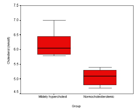
(C) Side-by-side boxplots

Group 1 calculations:

5.8 5.8 5.8 5.9 6.0 6.0 | 6.1 6.3 6.4 6.5 6.7 7.0 Q0 Q1 Q2 Q3 Q4

The median (Q2) has a depth of (12+1)/2 = 6.5 placing it between 6.0 and 6.1. Average these values to derive a median (Q2) of 6.05.
Q1 is calculated as follows: n_{bottom half} = 6. The hinge of the bottom half (Q1) has a depth of = (6+1)/2 = 3.5, thus falling between the 5.8 and 5.9 (Q1 = 5.85).
Q3 falls between 6.4 and 6.5 and is thus 6.45.
The five-point summary is: 5.8, 5.85, 6.05, 6.45, 7.0
IQR = 6.45 - 5.85 = 0.6
F_U = 6.45 + (1.5)(0.6) = 7.35. (No values above the fence, so the top whisker point is 7.0.)
F_L = 5.85 - (1.5)(0.6) = 4.95. (No values below the bottom fence, so the bottom whisker point is 5.8.)

Group 2 calculations:

4.7 4.8 4.9 5.3 5.3 5.4 Q0 Q1 Q2 Q3 Q4

The 5-point summary is 4.7, 4.8, 5.1, 5.3, 5.4
IQR = 5.3 - 4.8 = 0.5
F_U = 5.3 + (1.5)(0.5) = 6.05 (no outside values--top whisker goes to maximum)
F_L = 4.8 - (1.5)(0.5) = 4.05 (no outside values--bottom whisker goes to minimum)

The side-by-side plots:

(D) SPSS Analysis (p. 13)

Descriptive statistics from SPSS

The first part of the output is:

This is how we confirm the sample sizes of the groups.

The second part reports summary statistics. Notice that the EXPLORE command's interquartile range is slightly different than the IQR reported by hand. This is because there are several ways to interpolate quartiles. We use Tukey's hinges. SPSS uses weighted percentiles when calculating its interquartile range. Other calculations in the output should match your hand calculations.

The side-by-side boxplots are shown above.

(E) F-ratio test (p. 14)
H₀: s₁² = s₂²
H₁: s₁² s₂²

F_stat = (.392)² / (.301)² = 1.69
df₁ = 12 - 1 = 11
df₂ = 6 - 1 = 5

The p value is the area under the curve to the right of 1.69 on the F_11,5 distribution. The landmark on the F table is F_11,5,.95 = 4.70. Therefore, p > .05. Using StaTable we get p = .29. H₀ is retained; there no significant difference in variances (i.e., the differences in sample standard deviations -- .39 vs. .31 -- may merely be random. It seems reasonable to proceed under an assumption of homoscedasticity.

(F) Testing the mean difference (p. 15)

H₀: �₁ = �₂
H₁: �₁ �₂

Equal variance t test statistic
s²_p = [(.392² )(11) + (.301²)(5)] / 16 = 0.134
se_{mean dif} = [(.134)(1/12 + 1/6)] = 0.183
t_stat = (6.192 - 5.067) / 0.183 = 6.15
df = 11 + 5 = 16
p < .001 (p = 1.4E-0005 by computer)
Conclude: reject H₀
The difference in means is "significant."

Unequal variance ttest statistic
se_{mean dif} = (.392² / 12 + .301² / 6) = 0.167
t_stat = (6.192 - 5.067) / 0.167 = 6.73
df by conservative hand-based method = 5 (using full formula df'' = 12.9)
p < .002
Conclude: reject H₀ (observed difference in means is "significant")

(G) Replicate analysis in SPSS and answer questions (p. 16)

Output from SPSS Compare Means > Independent Samples T test command

What is the p value derived by Levene's test of equal variance? p = .451

What is the p value derived by F ratio test [done by hand, p. 14]? p = .58

How do these p values compare? Do the conclusions that follow differ? No. Both p values are "large", and both retain the null hypothesis of "equal variance."

What is the p value derived by the equal variance t test? p = .000

What is the p value derived by the unequal variance t test? p = .000

How do these p values compare? Do the conclusions that follow differ? Both p values are very small (less than .0005). Both provide evidence to reject the null hypothesis.