[2] Interpretation states that scatter plot reveals a positive linear relation between,
and no outliers are evident. {You cannot determine "strength"
from a scatter plot -- axis scaling will skew interpretation}
(14.2) ANSCOMBE The correlation coefficient should be disregarded in all but case I. (Correlation is not warranted in case II because the relation between X and Y is not linear. Correlation is not warranted in case III because of the outlier. In case IV, there is no variation in X except for the outlier in the upper-right quadrant.)
(14.4) NA-BP
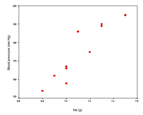
(A)
| [1] Scatterplot is accurate and labeled.
[2] Interpretation states that scatter plot reveals a positive linear relation between,
and no outliers are evident. {You cannot determine "strength"
from a scatter plot -- axis scaling will skew interpretation} |
|
[3] (B)
r = 26.18 / sqrt [(0.409)(1979.60)] = 0.9201 @
0.92 {APA requires two decimals}
[4] Strong positive correlation.
[5] r2 = 0.8464 @ 0.85,
indicating that 85% of the variation in Y is "explained" by variation in
X.
[6] (C) Test of H0: r = 0
[7] ser = sqrt[(1 - 0.8464) /8] =
0.1386
[8] tstat = (.920 ) / 0.1386 = 6.64; df = 10 - 2 =
8
[9] p = .00016
[10] Yes. The correlation is significant at alpha = .01.
{It is good to practice a make a brief holistic summary of your analysis: The
observed linear relation is strong, positive, and
statistically significant.}
(14.8) MAT-MORT.SAV - A brief answer key is provided FYI. Scatterplot not shown so key will fit on a single page, but should be accurate with X and Y labeled. Interpretation should mention that the relation is linear and negative. No outliers are evident. Correlation coefficient: r = -.90; This indicates a strong negative correlation. Test of H0: r = 0; tstat = 6.19, df = 9, p = .00016, indicating significance at conventional levels. The observed correlation is linear, strong, negative, and significant.