Jump to lab: 1 | 2 | 3 | 4 | 5 | 6 | 7 | 8 | 9 | 10
1. Random numbers.
My random numbers below were generated Aug 2001 using www.random.org. Sampling was done with replacement.
|
first |
80 |
|
second |
485 |
|
third |
15 |
|
fourth |
43 |
|
fifth |
419 |
|
sixth |
531 |
|
seventh |
351 |
|
eighth |
327 |
|
ninth |
219 |
|
tenth |
546 |
2. Data / hand-written table.
| id | age | sex | date | hiv | sbp1 | sbp2 |
| 80 | 21 | F | 1/9/04 | 2 | 120 | 126 |
| 485 | 42 | M | 10/21/04 | 2 | 118 | 118 |
| 15 | 5 | M | 1/12/05 | 2 | 83 | 86 |
| 43 | 11 | F | 2/17/04 | 1 | 126 | 124 |
| 419 | 30 | M | 12/28/04 | 2 | 119 | 118 |
| 531 | 50 | M | 12/29/04 | 2 | 114 | 118 |
| 351 | 28 | M | 8/19/04 | 2 | 119 | 119 |
| 327 | 27 | M | 8/31/04 | 2 | 115 | 111 |
| 219 | 24 | M | 8/19/04 | 2 | 127 | 129 |
| 546 | 52 | M | 10/13/04 | 2 | 94 | 89 |
3. Variable names and types.
4. Data entry.
1. Stem-and-leaf plots
a. Single stem-values
|0|5
|1|1
|2|1478
|3|0
|4|2
|5|02
x10
b. Split stem-values
|0|5
|1|1
|1|
|2|14
|2|78
|3|0
|3|
|4|2
|4|
|5|02
x10
c. Which of the above plots do you prefer? Plot A. Why? It does a better job showing the shape of the distribution. [Reasonable interpretations of your own data.]
d. My distribution has a mound, no pronounced skew, and no apparent outliers. (Keep in mind that with small data sets, it is difficult to make reliable statements about the shape of a distribution. We offer this analysis for practice purposes only.
e. The mean looks to be in the high 20s or low 30s
f. Data spread from 5 to 52.
2. SPSS stemplot
3. Frequency Table
a. By hand
|
Age (years) |
Frequency Count |
Relative Freq (%) |
Cumulative Freq (%) |
|
0!9 |
1 |
10 |
10 |
|
10!19 |
1 |
10 |
20 |
|
20!29 |
4 |
40 |
60 |
|
30!39 |
1 |
10 |
70 |
|
40!49 |
1 |
10 |
80 |
|
50!59 |
2 |
20 |
100 |
|
|
10 |
100 |
-- |
b. Tallied with SPSS AGEGRP coded 1 = 0 - 9, 2 = 10 - 19, and so on.
|
|
Code |
Frequency |
Percent |
Valid Percent |
Cumulative Percent |
|
Valid |
0 |
1 |
10.0 |
10.0 |
10.0 |
|
|
1 |
1 |
10.0 |
10.0 |
20.0 |
|
|
2 |
4 |
40.0 |
40.0 |
60.0 |
|
|
3 |
1 |
10.0 |
10.0 |
70.0 |
|
|
4 |
1 |
10.0 |
10.0 |
80.0 |
|
|
5 |
2 |
20.0 |
20.0 |
100.0 |
|
|
Total |
10 |
100.0 |
100.0 |
|
c. Optional -- SPSS recode command
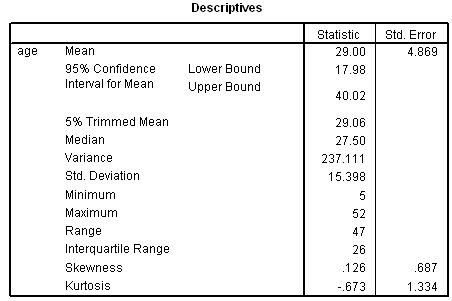
1. Sample mean
a. n = 10; Sum(x)
= 290; ![]() = (1 / n) � Sum(x)
= (1 / 10) � 290 = 29.0
= (1 / n) � Sum(x)
= (1 / 10) � 290 = 29.0
b. Uses of the sample mean
(i) Predict s a value selected at random from the sample
(ii) Predicts a value selected at random from population
(iii) Predicts the population mean
2. Variance and standard deviation
a. Deviations table
| i | x | deviation | sq deviation |
| 1 | 21 | -8 | 64 |
| 2 | 42 | 13 | 169 |
| 3 | 5 | -24 | 576 |
| 4 | 11 | -18 | 324 |
| 5 | 30 | 1 | 1 |
| 6 | 50 | 21 | 441 |
| 7 | 28 | -1 | 1 |
| 8 | 27 | -2 | 4 |
| 9 | 24 | -5 | 25 |
| 10 | 52 | 23 | 529 |
| Sums | 290 | 0 | 2,134 |
b. SS = sum of last column = 2134
Comment: Here is how this formula looks in horizontal fashion: (21 - 29)� + (42 - 29)� + (5 - 29)� + (11 - 29)� + (30 - 29)� + (50 - 29)� + (28 - 29)� + (27 - 29)� + (24 - 29)� + (52 - 29)�
c. s2 = 2134 / (10 -
1) = 237.1111 (years2)
d. s = /(237.1111)
= 15.3984 ![]() 15.4
years
15.4
years
e. 95% of the data
will lie within two standard deviations of the mean when the distribution is
Normal.
f. ...at least 75% of the values will lie within 2 standard deviations of the mean.
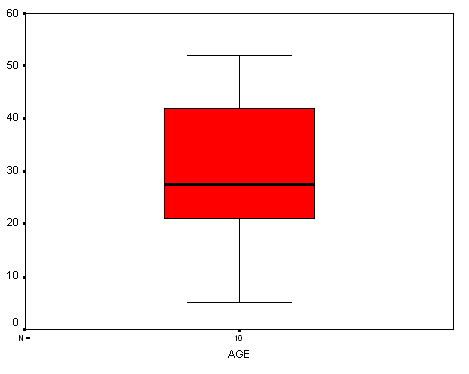
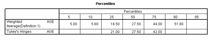
3. Quartiles and boxplot
Ordered Array:
5 11 21 24 27 | 28 30 42 50 52
low group
| high group
Five point summary: 5, 21, 27.5, 42, 52
IQR = 42 - 21 = 21
FU = 42 + (1.5)(21) = 73.5; hence, no upper outside values and upper inside value = 52.
FL = 21 - (1.5)(21) = -10.5; hence no lower outside values and The lower inside value = 5
Boxplot
4. SPSS

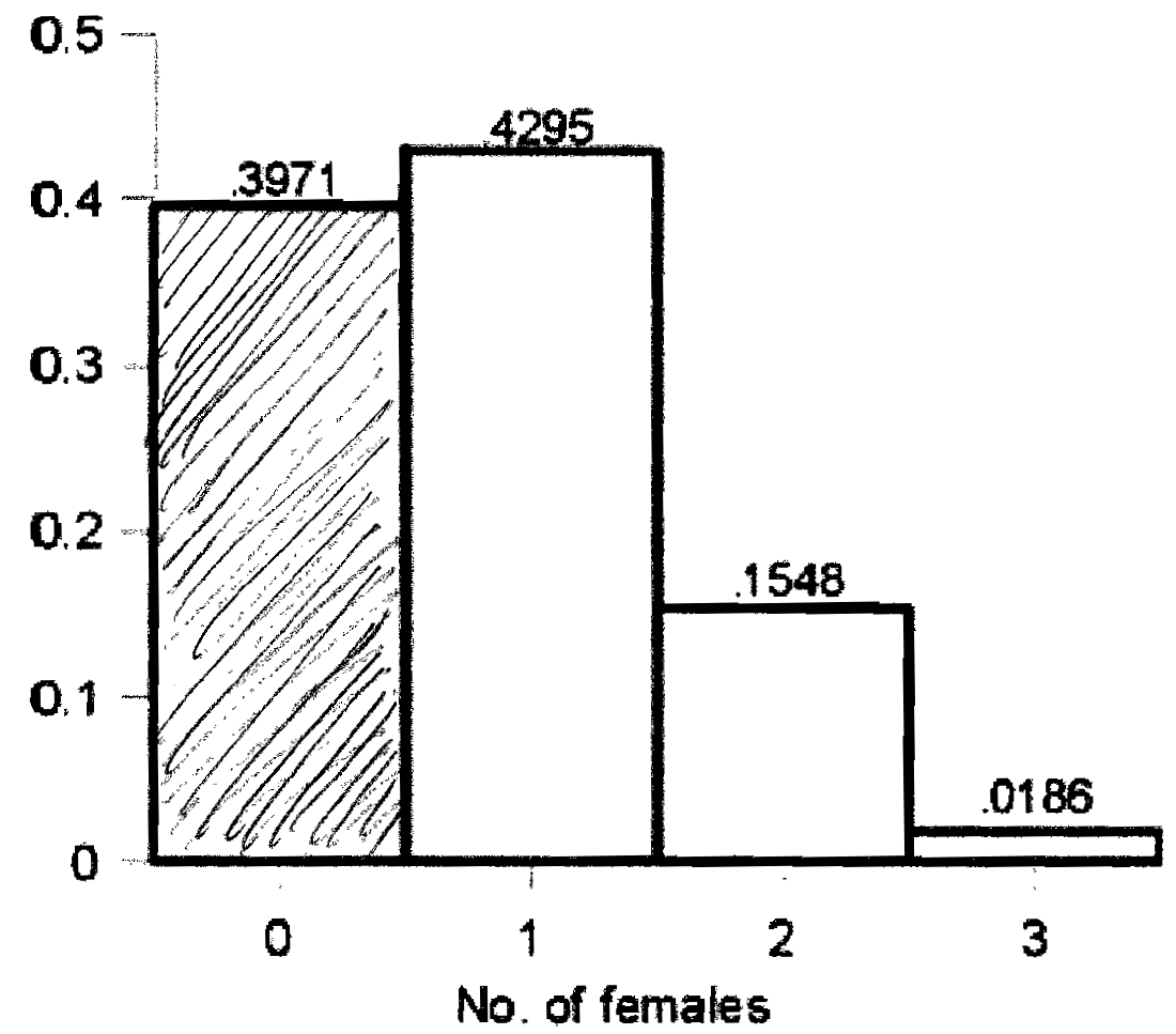
1. Introduction to the binomial.
n = 3
p = 0.265
2. Mean and standard deviation.
a. μ = np =
3 � 0.265 = 0.795
b. ![]() = sqrt(npq)= sqrt(3 � 0.265 � 0.735) = 0.7644
= sqrt(npq)= sqrt(3 � 0.265 � 0.735) = 0.7644
3. Choose function [binomial coefficients]
a. 3C0 = 3! / [(0!)(3 - 0)!] = (3 � 2
� 1) / [(1)(3 � 2 � 1)] = 1
b. 3C1 = 3! / [(1!)(3 - 1)!] = (3 � 2
� 1) / [(1)(2 � 1)] = 3
c. 3C3 = 3! / [(3!)(3 - 3)!] = (3 � 2
� 1) / [(3 � 2 � 1)(1)] = 1
4. [Binomial probabilities].
a. q = 1 - .265 = .735
b. Pr(X = 0) = (3C0)(0.2650)(0.7353-0)
= (1)(1)(0.3971) = 0.3971
c. Pr(X = 1) = (3C1)(0.2651)(0.7353-1)
= (3)(0.2650)(0.5402) = 0.4295
d. Pr(X = 2) = (3C2)(0.2652)(0.7353-2)
= (3)(0.0702)(0.7350) = 0.1548
e. Pr(X = 3) = (3C3)(0.2653)(0.7353-3)
= (1)(0.0186)(1) = 0.0186
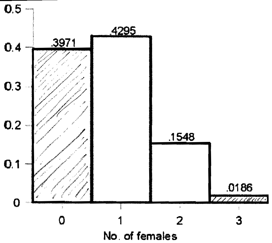
5. Area under the curve.
a. Shade bar corresponding to Pr(X = 0)
b. Shade bar corresponding to Pr(X = 3)

This AUC = .0186 � 1 = .0186
c. Pr(X = 0) + Pr(X = 3) = 0.3971 + .0186 = .4157
Visually:
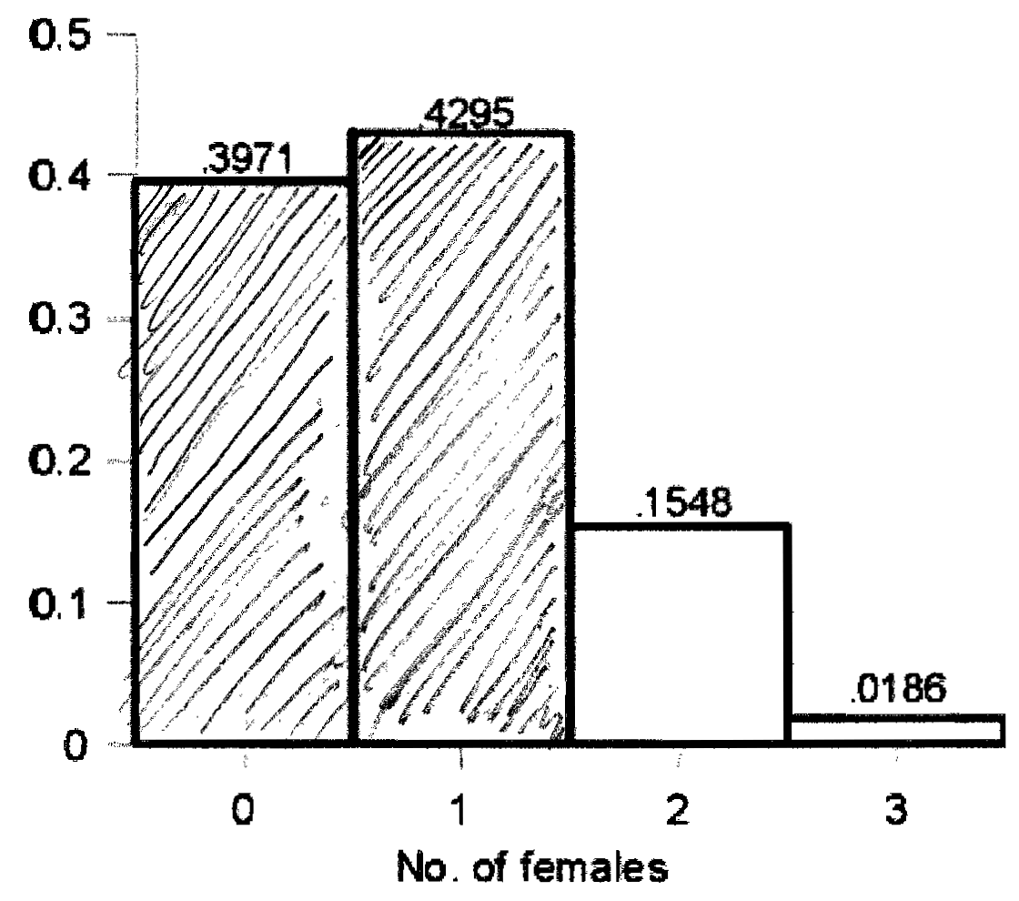
6. Cumulative probabilities
a.
Pr(X ![]() 0) = 0.3971
0) = 0.3971
b. Pr(X ![]() 1) = 0.3971 + 0.4295 = 0.8267
1) = 0.3971 + 0.4295 = 0.8267
c. Pr(X ![]() 2) = 0.8267 + 0.1548 = 0.9815
2) = 0.8267 + 0.1548 = 0.9815
d. Pr(X ![]() 3) = 0.9815 + 0.0186 = 1.0000
3) = 0.9815 + 0.0186 = 1.0000
e. Shaded area corresponding to Pr(X ![]() 1) = (0.3971 � 1.0) + (0.4295 � 1.0) = 0.8267
1) = (0.3971 � 1.0) + (0.4295 � 1.0) = 0.8267
7. Right tail.
a. Shade area corresponding to Pr(X > 1)
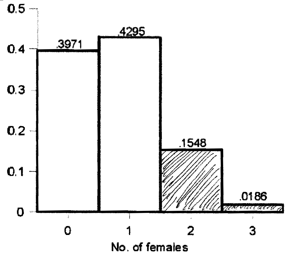
b. Pr(X > 1) = Pr(X = 2) + Pr (X = 3) = 0.1548 + 0.0186 = 0.1733
c. Pr(X > 1) = 1 - Pr(X ![]() 1) = 1 - 0.8267 = 0.1733
1) = 1 - 0.8267 = 0.1733
8. Use of StaTable binomial probability calculator (optional/recommended).
1. Introduction
2. X ~ N(120, 20)
a. Label � with 120
b. Label � � ![]() markers with 100 and 140.
markers with 100 and 140.
c. Label
� � 2![]() markers with 80 and 160
markers with 80 and 160

d. 95%
3. Standard Normal random variable
a. z = (80 - 120) / 20 = -2
b. z = (80 - 100) / 20 = -1
c. z = (160 - 120) / 20 = 2
4.Normal probabilities:
a. Note
steps...
State: Pr(X ![]() 100)
100)
Standardize: z = (100 - 120) / 20 = -1
Sketch: not shown
Table B: Pr(Z ![]() -1)
= .1587
-1)
= .1587
b. Pr(X > 100) = Pr(Z >1)
= 1 - Pr(Z ![]() 1)
= 1 - .1587 = 0.8413
1)
= 1 - .1587 = 0.8413
1. Population & sample
a. ![]() = 29.0 (unique to Dr.
Gerstman's sample)
= 29.0 (unique to Dr.
Gerstman's sample)
b. The ![]() s differs because of random [sampling] variation.
s differs because of random [sampling] variation.
c. Ways ![]() and � differ (p. 157)
and � differ (p. 157)
(1) different sources - sample vs. population
(2) ![]() is calculated in the sample, �
is
not
is calculated in the sample, �
is
not
(3) ![]() is a random variable, � is a
constant
is a random variable, � is a
constant
(4) different notation (obvious but important)
2. Experiment simulation
As of September 2003, the distribution looked like this. (This distribution will change over time, as additional student means are added to the data.)
a. The mean of the SDM was 29.4 (as of September 2003; will change)
b. Standard deviation of the SDM was 4.05 (as of September 2003; will change)
c. More Normal.This table reviews the different distributions that students should keep in mind during the lab (not part of lab manual, but good review in case a student is confused.)
|
Various distributions considered in this lab: |
Population |
Sample |
Simulated SDM |
|
Number of observations |
N = 600 |
n = 10 |
changes as data accrues |
|
mean |
� = 29.5 |
|
changes but should approach 29.5 as study continues |
|
standard deviation |
s = 13.59 |
s varies from sample to sample |
changes but should approach 4.3 as study continues |
3. SDM model, right tail
a. 2.5%
b. The theory performed well. It predicted that between 2 and 3 sample
means would exceed 38. This turned out to be true.
4. Confidence interval for m, sigma known
a. No answer required; the question gives SE =
![]() /
/ ![]() n =
13.59 /
n =
13.59 / ![]() 10 =
4.30.
10 =
4.30.
b. ![]() � (1.96)(SE) = 29.0 �
(1.96)(4.30) = 29.0 � 8.4 = 20.6 to 37.4
� (1.96)(SE) = 29.0 �
(1.96)(4.30) = 29.0 � 8.4 = 20.6 to 37.4
c. This particular CI did capture �
d. 5%
e.29.0 � (1.645)(4.30) = 29.0 � 7.1 = 21.9 to 36.1
f. 29.0 � (2.576)(4.30) = 29.0 � 11.1 = 17.9 to 40.1
g. It increased.
5. Hypothesis test
a. H0: m = 32 versus
Ha: m ![]() 32
32
b. zstat = (![]() - �0) / SE = (29.0 - 32) / 4.30 =
-0.70
- �0) / SE = (29.0 - 32) / 4.30 =
-0.70
c. The curve should accurately show the location of the student's zstat
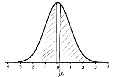
with the tail of the distribution shaded. Dr. Gerstman's one-tailed P = Pr(Z < -0.70) = 0.2420
d. Two-tailed P = 0.4840 [
e. My test provides statistically nonsignificant evidence against the null hypothesis.
(Comment: Retention of the false null hypothesis would result in a type II error.
This is one of the key limitations of statisical hypothesis testing.)
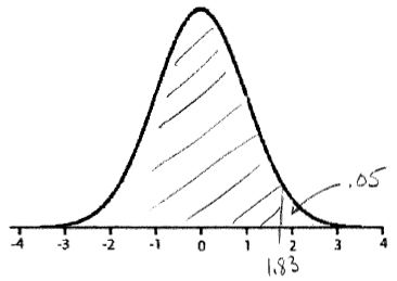
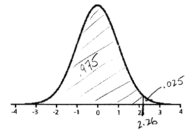
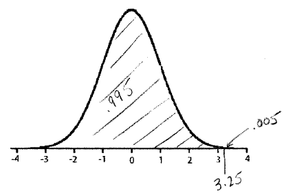
1. Student's pdf
a. t9,.95 = 1.83; right tail = 0.05
b. t9,.975 =2.26; right
tail = 0.025
c. t9,.995 = 3.25; right tail = 0.005
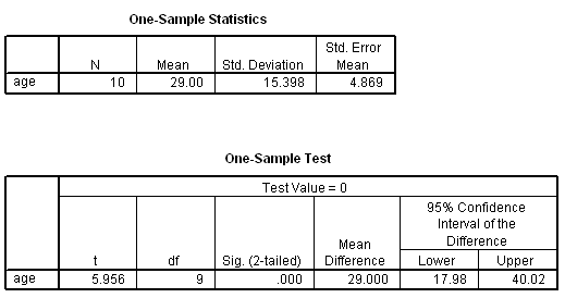
2. t Confidence Interval
a. The standard deviation
of AGE in GerstmanB10.sav is 15.398
b. SE = s / ![]() n
= 15.398 /
n
= 15.398 / ![]() 10 =
4.8693
10 =
4.8693
c. 95% confidence interval for μ = ![]() � (t9,.975)(SE)
= 29.00 � (2.262)(4.869) = 29.00 � 11.01 = (18.0, 40.0).
� (t9,.975)(SE)
= 29.00 � (2.262)(4.869) = 29.00 � 11.01 = (18.0, 40.0).
Comment: This confidence interval suggests the population mean age is between 18 and 40.
3. SPSS.
4. Paired samples
a. These are paired samples because each data point in sample one is uniquely paired to a data point in sample two.
b. Data
SBP1 SBP2 DELTA
120 126 -6
118 118 0
83 86 -3
126 124 2
87 82 5
114 118 -4
119 119 0
115 111 4
127 129 -2
94 89 5
c. Stemplot (including interpretation)
-1|
-0|6
-0|432
0|0024
0|55
1|
�10 (DELTA)
d. Descriptive
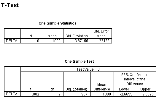
statistics for delta variable: ![]() = 0.1 s = 3.87155
n = 10
= 0.1 s = 3.87155
n = 10
e. Hypothesis test
H0:
md
= 0 versus Ha: md ![]() 0
0
tstat = (0.100 - 0) / 1.224 = 0.08; df =
10 - 1 = 9
One-sided P > 0.25;
two-sided P > 0.50 (two-sided P ![]() .92 using Table G)
.92 using Table G)
The evidence against the hypothesis is not statistically significant.
5. SPSS
6. Power of the test (optional)
a. Power = ![]() [-1.96+(5
�
[-1.96+(5
� ![]() 10 / 5)] =
10 / 5)] = ![]() (1.20) =
0.8849 = 88.5%
(1.20) =
0.8849 = 88.5%
b. Power = ![]() [-1.96+(2
�
[-1.96+(2
� ![]() 10 / 5)] =
10 / 5)] = ![]() (-0.70) =
0.2420 = 24.2%
(-0.70) =
0.2420 = 24.2%
c. Lowering the difference worth detecting decreased the power of the
study (making it more difficult to detect the difference).
d. Power = ![]() [-1.96+(2
�
[-1.96+(2
� ![]() 50 / 5)] =
50 / 5)] = ![]() (0.87) =
.8078 = 80.8%
(0.87) =
.8078 = 80.8%
e. Increasing the sample size increased the power of the test.
1. Data
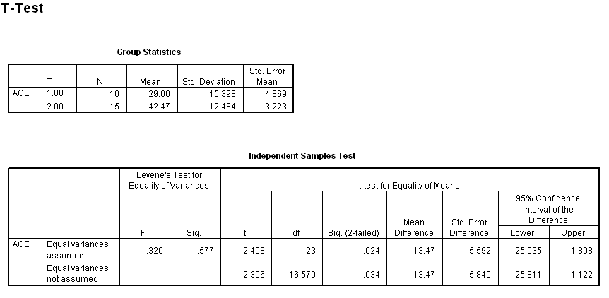
a. Summary statistics for the AGE variable in GerstmanB10.sav:
n1 = 10 ![]() 1
= 29.00 s1 = 15.40
1
= 29.00 s1 = 15.40
b. Summary statistics for group 2 (given in the problem): n2 = 15 ![]() 2
= 42.47 s2 = 12.48
2
= 42.47 s2 = 12.48
2. Estimation
a. ![]() 1 -
1 - ![]() 2 = 29.00 - 42.47 =
-13.47. Group 2 has the higher average by 13.47 years.
2 = 29.00 - 42.47 =
-13.47. Group 2 has the higher average by 13.47 years.
b. SE = 5.840
c. dfconserv = 9
d. 95% confidence interval for �1 - �2 = ![]() 1 -
1 - ![]() 2 � (t9,.975)(SE) = -13.47 �
(2.262)(5.840) = -13.47 � 13.21 = (-26.68 to -0.26 ) SE and mean difference
should match, but CI will be a little wider (more conservative) than SPSS
confidence interval for "equal variance not assumed method".
2 � (t9,.975)(SE) = -13.47 �
(2.262)(5.840) = -13.47 � 13.21 = (-26.68 to -0.26 ) SE and mean difference
should match, but CI will be a little wider (more conservative) than SPSS
confidence interval for "equal variance not assumed method".
e. The interpretation should address the fact that the CI is trying to capture �1 - �2
with 95% confidence.
3.Hypothesis test
a. H0: μ1 - μ2 = 0
versus Ha: μ1
- μ2 ![]() 0
0
b. tstat = (29.00 - 42.47) / 5.840 = -2.31 with dfconserv = 9
c. P-value based on t sampling distribution
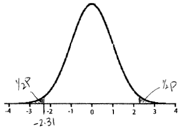
Two-sided P-value
![]() 0.047 via Table G.
The hand-calculated results will be
close but not identical to the "equal variance not assumed" t
test results produced by SPSS.
0.047 via Table G.
The hand-calculated results will be
close but not identical to the "equal variance not assumed" t
test results produced by SPSS.
Interpretation: Data provide significant evidence against H0.
4. SPSS
5. Conditions. Graphical methods such as stemplots can be used to address Normality.. In practice, it is enough that the two distribution have similar shapes and no strong outliers.With small samples it is very difficult to check for Normality.
1. Sample size requirement Make sure this problem is done accurately.
a. n = (1.96)2(0.5)(0.5) / 0.12 @ 96.04; use 97
b. n = (1.96)2(0.5)(0.5) / 0.052 @ 384.16; use 385
c. n = (1.96)2(0.5)(0.5)
/ 0.0252
@ 1536.64; use 1537
d. The sample size requirement quadruples.
2. New data set: population2.sav
3. SPSS tabulation Make sure this problem is properly done.
x = 66
n = 600
4. Estimation Make sure this problem is done in its entirety.
a.
![]() = 66 / 600 = .110 or 11.0%
= 66 / 600 = .110 or 11.0%
b. Confidence interval for p: Note that p~ = 68 / 604 = .1126; q~ = .8874; SEp~ = .01286.
95% CI = .1126 � (1.96)(.01286) = .1126 � .0252 = (.0874 to .1379)
Interpretation: Based on these data we can be 95% confident that the parameter (proportion in the source population) is between 8.8% to 13.8%.
5. One-sample z test of the proportion Make sure this problem is done in it's entirety.
a. H0: p = 0.10 vs. Ha: p
![]() 0.10
0.10
b. SE = .01225; zstat = (0.11 -
0.1) / .01225 = 0.82
c.

P-value = 0.412; The evidence against H0 is not significant.
d. The 95% confidence interval captured the value hypothesized by the null (i.e., p0 = .10). Thus, the test of of H0: p = 0.10 will not be significant at the alpha = .05 level. (i.e., P > .05).
6. WinPepi. The WinPepi results are shown in the lab workbook.
1. Cross-tabulation
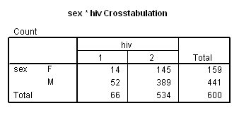
2. Estimation
a. Prevalences and prevalence ("risk") difference:
Prevalence females = ![]() 1 = 14 / 159 = .08805
1 = 14 / 159 = .08805
Prevalence in males = ![]() 2 = 52 / 441 = .1179;
2 = 52 / 441 = .1179;
![]() 1 -
1 - ![]() 2
= .08805 - .1179 = -0.02985
2
= .08805 - .1179 = -0.02985
Interpretation: The prevalence in females in the sample is 3.0% less than in males.
b. 95% confidence interval for p1 - p2
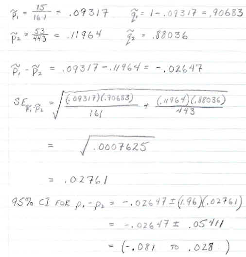
Note: Using WinPepi, the 95% CI by Wilson's method is -0.078 to 0.031.
3. Hypothesis test
a. H0: p1
= p2 versus Ha: p1 ![]() p2 (equivalently, H0:
p1 - p2 = 0 versus Ha:
p1 - p2
p2 (equivalently, H0:
p1 - p2 = 0 versus Ha:
p1 - p2 ![]() 0)
0)
b.

zstat = 1.03
c. P = 0.302
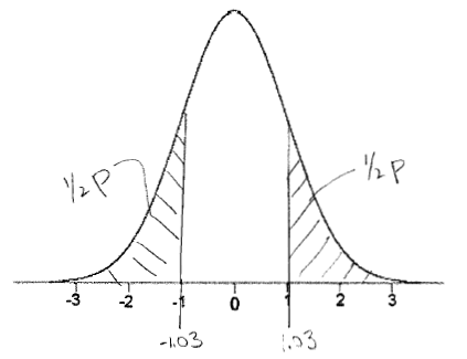
d. The evidence against H0 is not
significant ("no significant difference in prevalence by gender"). Discuss the results in
your own words.
4. WinPepi. (optional)