17: Odds Ratios from Case-Control Studies version: 9/23/06

Review Questions

1. How do case-control studies differ from cohort studies?
2. Why are case-control studies unable to estimate incidence or prevalence?
3. What symbol is used to denote the odds ratio parameter? What symbol is used to denote the odds ratio estimator?
4. Before calculating a confidence interval for the odds ratio, we converts the odds ratio estimate to a ______________ scale.
5. List the null hypothesis tested by case-control data.
6. When is Fisher's test used in place of a chi-square test?
7. In a  2-by-2 table for  matched-pair data, table cells t and w contain counts for ____________ pairs, while cells u and v contain counts for ___________ pairs.
8. True or false? In matched case-control studies, information about concordant pairs is ignored.
9. What is the name of the chi-square statistic used to test matched-pair data?
10. What is the primary benefit of matching?
11. [T or F?] You can use a 95% confidence for the odds ratio to determine statistical significance at alpha = 0.05.
12. [T or F?] You can use a 95% confidence for the odds ratio to determine statistical significance at alpha = 0.01.
13. How do you use a 95% confidence for the odds ratio to determine statistical significance at alpha = 0.05?
14. Which of the following 95% confidence interval for odds ratios are significant at alpha = 0.05? (a) 0.01 to 0.77 (b) 0.77 to 1.23 (c) 1.23 to 2.43

Exercises

Part A: Independent Samples

17A.1 Wynder and Graham's case-control study of smoking and lung cancer. A historically important study published compared the smoking histories of 605 cases with lung cancer to 780 controls without cancer. Data on average use of tobacco during the past 20 years was classified as follows:

• 5 = Chain smoker (35 cigarettes of more per day for at least 20 years)

• 4 = Excessive smoker (21 � 34 cigarettes per day for more than 20 years)

• 3 = Heavy smoker (16 � 20 cigarettes per day for more than 20 years)

• 2 = Moderately heavy smoker (10 � 15 cigarettes per day for more than 20 years)

• 1 = Light smoker (1 � 9 cigarettes per day for more than 20 years)

• 0 = Non-smoker (less than 1 cigarette per day for more than 20 years)

 If the patient smoked for less than 20 years, the amount of smoking was reduced in proportion to its duration.

Cross-tabulation revealed (Wynder & Graham, JAMA, 1950. click names for biographies; click citation for article reprint): 

Smoking	Cases	Non-cases
5	123	64
4	186	98
3	213	274
2	61	147
1	14	82
0	8	115
Total	605	780

Calculate odds ratio for each level of smoking using the non-smokers as the reference group. (Optional: Determine 95% confidence intervals for each estimate.) Interpret these results. 

17A.2 Cell phone use and brain tumors. Results from two case-control studies on cell phone use and brain cancer are summarized below. Review each summary and discuss whether the study in question supports or does not support the theory that recent use of hand-held cellular telephones causes brain tumors. Explain your reasoning in each instance.

(A) A case-control study by  Inskip and co-workers (2001) examined the use of cellular telephones between 1994 and 1998 in 782 cases with various forms on intracranial tumors and 799 controls admitted to the same hospitals for a variety of nonmalignant conditions. Subjects were considered exposed if they reported use of a cellular telephone for more than 100 hours. The odds ratio (OR) for glioma was 0.9 (95 percent confidence interval 0.5 to 1.6), the OR for meningioma  was 0.7 (95 percent confidence interval 0.3 to 1.7), the OR for acoustic neuroma 1.4 (95 percent confidence interval 0.6 to 3.5), and the OR for all tumor types combined: 1.0 (95 percent confidence interval 0.6 to 1.5)

(B)  A case-control study by Muskat and co-worker (2000)[full text] conducted between 1994 and 1998 used a structured questionnaire to quantify the statistical relation between cell phone use and primary brain cancer in 469 cases and 422 matched controls. The results of the study stated "The median monthly hours of use were [sic] 2.5 for cases and 2.2 for controls. Compared with patients who never used handheld cellular telephones, the multivariate odds ratio (OR) associated with regular past or current use was 0.85 (95% confidence interval [CI], 0.6-1.2). The OR for infrequent users (<0. 72 h/mo) was 1.0 (95% CI, 0.5-2.0) and for frequent users (>10.1 h/mo) was 0.7 (95% CI, 0.3-1.4). The mean duration of use was 2.8 years for cases and 2.7 years for controls . ..  The OR was less than 1.0 for all histologic categories of brain cancer except for uncommon neuroepitheliomatous cancers (OR, 2.1; 95% CI, 0.9-4.7)."

17A.3 Esophageal cancer and tobacco consumption (dichotomized exposure). This exercise considers tobacco use with exposure dichotomized at 20 gms/day on the risk of esophageal cancer in the bd1.sav data set (right-click data set name to download file). Data are originally from Tuyns and coworkers (1977) as reported by Breslow and Day (1980). Cross-tabulation reveals:

(A) Calculate the odds ratio and its 95% confidence interval. Interpret your result. 
(B) Using a chi-square statistic, derive a P-value for the problem.
(C) Download bd1.sav (right-click > Save as). After downloading the file, open it in SPSS and print the code book by clicking File > Display Data Info > bd1.sav > OK. Keep the codebook handy for future reference. 
(D) Cross-tabulate the data by clicking Analyze > Descriptive Statistics > CrossTabs. Select TOB2 as the row (exposure) variable and CASE as the column (outcome) variable. Click the statistics button and check the boxes for Chi-square and Risk . Click Continue > OK. Do the results in SPSS confirm your earlier calculations?

17A.4 The Oxford Childhood Cancer Survey. The file bd2.sav contains data from a case-control study on childhood leukemia and in utero X-ray exposure (Breslow & Day, 1980, p. p. 240). Cases are children less than 10 years of age with leukemia or lymphoma occurring in the period 1954-65. Controls are similarly aged children from the same neighborhood. Data are stored in the variable CASE: (1 = case, 2 = control). In utero exposure to diagnostic radiography is stored in the variable XRAY: (1 = yes, 2 = no). [Original data are matched-pairs. We have ignored the match. In practice, ignoring the match is not recommended but this instance, makes little difference in risk estimates.]

(A) Download the dataset  bd2.sav  and then cross-tabulate the data. Show data as a 2-by-2 table XRAY as the row variable and CASE as the column variable.
(B) Calculate the odds ratio and its 95% confidence interval. Interpret your findings. Do data support the hypothesis that in utero X-ray exposure increases the likelihood of childhood leukemia & lymphoma? 
(C) Perform a chi-square test of H₀:y  = 1. 

17A.5 Doll & Hills, 1950.  A historically important case-control study of smoking and carcinoma of the lung was completed by Doll & Hill in 1950. They found 647 of the 649 lung cancer cases were smokers compared with 622 of 649 controls. (Click here for a reprint of the original article.) Display thee data in 2-by-2 crosstab and calculate the odds ratio. Include a 95% confidence interval for the odds ratio parameter, and interpret your results 

17A.6  IUDs  and infertility. A case-control study of contraceptive devices and infertility found prior use of intra-uterine devices (IUDs) in 89 of 283 infertile cases. In contrast, 640 of 3833 fertile control women had used IUDs (Cramer et al., 1985; Rosner, 1990, p. 381).  Data are shown in a 2-by-2 table, below. Calculate the odds ratio and its 95% confidence interval. Interpret the results.

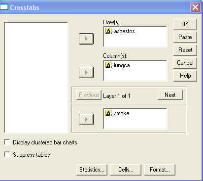
17A.7 Asbestos, cigarettes, and lung cancer. Data stored in asbestos.sav are from a case-control study on lung cancer, asbestos  exposure, and smoking. Right-click the file name to download the dataset. By going through the steps listed below, you will learn about interaction. 

(A) Cross-tabulate LUNGCA (column variable) by SMOKE (row variable). Determine the odds ratio.
(B) Cross-tabulate LUNGCA by ASBESTOS. Determine the odds ratio.
(C) Cross-tabulate LUNGCA by ASBESTOS stratified by by SMOKE. This is accomplished by filling in the SPSS dialogue box shown below. Calculate odds ratios separately for smokers and non-smokers. Are these odds ratios homogeneous or heterogeneous? 

17A.8 Esophageal cancer and alcohol recorded at four levels. This data set was introduced in StatPrimer. In StatPrimer, alcohol consumption was dichotomized at 80 g/day. However, data were initially recorded at four different levels of alcohol consumption (0-39, 40-79, 80-119, 120+). You can calculate the odds ratio associated with these increasing levels of exposure by comparing each exposure level to the baseline provided by the least exposed group. Calculate the odds ratio for each table below and interpret the results. Is there evidence of a dose-response relationship? 

Low vs. very low alcohol consumption
gms/day   Cases   Controls
40-79      75      280
0-39       29      386

Intermediate vs. very low alcohol consumption
gms/day   Cases   Controls
80-119     51       87
0-39       29      386

High vs. very low alcohol consumption
gms/day   Cases   Controls
120+       45       22
0-39       29      386

17A.9 Vasectomy and prostate cancer. Data from a case-control study on vasectomy and prostate cancer are cross-tabulated below (Zhu et al., 1996). Calculate the odds ratio and its 95% confidence interval. (Optional: Calculate the P-value for the problem.)

17A.10 Brain tumors and electric blanket use. A case-control study assessed the risks of brain tumors associated with electric blanket use. Cross-tabulated data are shown below and are also stored as individual records in BRAINTUM.SAV (Preston-Martin et al., 1996). Calculate the odds ratio and its 95% confidence interval. Discuss the results.

17A.11 Baldness and the risk of heart attack. Both baldness and heart attacks are more common in males than in females. Is there a link between the two? The answer to this question takes on importance when treatments for baldness are considered. Minoxidyl, a treatment for baldness, is effective in some cases of male pattern baldness when applied topically. If the underlying condition of baldness elevates the risk of cardiovascular diseases, then any increase in the risk of cardiovascular disease in Minoxidyl users might mistakenly be attributed to the drug and not to the underlying condition of baldness. A study by Lesko and co-workers (1993) addressed this question by looking at data for 722 controls and 665 heart attack cases. Subjects were under 55 years of age who were admitted to hospitals in Massachusetts and Rhode Island. (Staff from the School of Public Health at the Boston University School of Medicine telephoned the hospitals to locate eligible cases.) Cases were men admitted for and survived a first heart attack with no prior serious heart problems. Controls were men admitted to the hospitals for non-fatal, non-cardiac problems. Control subjects with a prior history of heart disease were excluded from the study. Cases and controls were interviewed, and the degree of male pattern baldness was determined on a scale of 1 (no baldness) to 5 (extreme baldness). Data are cross-tabulated below: 

(A) Describe the association between baldness and heart attacks by either calculating exposure proportions in cases and controls or by calculating odds ratios associated with each level of baldness using baldness category 1 as the reference category.
(B) Conduct a chi-square test for overall association 
(C) Optional: Perform a test for trend. 
(D) Consider lurking variables that might explain the observed association, i.e., consider potential confounders. 

Baldness	Cases*	Controls
1 (none)	251	331
2	165	221
3	195	185
4	50	34
5 (extreme)	2	1
Total	663	772

Part B: Matched-pairs

17B.1 Fruits, vegetables, and adenomatous polyps. A case-control study by Witte and co-workers (1996) used matched-pairs to study the risk of adenomatous polyps of the colon in relation to diet. All cases and controls had undergone sigmoidoscopic screening. Controls were matched to cases on time of screening, clinic, age, and sex. One of the study's analyses considered the effects of low fruit and vegetable consumption on colon polyp risk. There were 45 pairs in which the case but not the control reported low fruit/veggie consumption. There were 24 pairs in which the control but not the case reported low fruit/veggie consumption [Summary counts reported in Rothman & Greenland, 1998, p. 287; same data used in StatPrimer as an illustrative example.]

(A) Calculate the odds ratio associated with low fruit/veggie consumption. Interpret this result. 
(B) Calculate a 95% confidence interval for the odds ratio. 
(C) Use a continuity-corrected McNemar statistic to calculate a P-value for the data.  
(D) Do data support the proposed connection between low fruit/veggie consumption and colon cancer?

17B.2 Smoking and mortality in identical twins. When smoking was first suspected as a cause of disease, Sir Ronald Fisher offered the constitution hypothesis as an explanation for the observed association. Fisher (1957, 1958a, 1958b) did not entirely dispose of the causal hypothesis, however.)  The constitutional hypothesis suggested that people genetically disposed to lung cancer were more likely to smoke. In other words, the relation between smoking and disease was confounded by constitutional factors. The constitutional hypothesis was put to the ultimate test by a study in which 22 smoking-discordant monozygotic twins where studied to see which twin first succumbed to death (Kaprio & Koskenvuo, 1989). In this study, the smoking-twin died first in 17 of the pairs (i.e., u = 17, while u + v = 22). Calculate the odds ratio for these data. Calculate a P-value for testing H₀: = 1. Interpret your findings. Which theory is refuted? Which is supported? [Same as StatPrimer illustrative example.]

17B.3 Collaborative Group Study of Stroke in Young Women, hemorrhagic stoke. The Collaborative Group Study of Stroke in Young Women (1975) was a case-control study of cerebrovascular disease and oral contraceptive use in women between 14- to 44-years of age completed in the 1970s. Cases were matched to neighborhood controls according to the age, sex, and race. 

(A) Here are the matched data for thrombotic stroke (Lilienfeld & Lilienfeld, 1980, p. 220). Calculate the odds ratio for these data.

Matched-pairs	Control exposed	Control non-exposed	Total
Case exposed	2	44	46
Case non-exposed	5	55	60
Total	7	99	106

(B) Suppose the match was broken and the investigators had analyzed the data unaware of the importance of matched-pair analyses. Rearrange the data in the above table to portray how it would look in an unmatched 2-by-2 cross-tabulation showing the number of exposed cases, exposed controls and so on. Then, calculate the odds ratio for these unmatched data. How does this compare to the results achieved with the proper matched analysis. 

17B.4 Collaborative Group Study of Stroke in Young Women, hemorrhagic stoke. Exercise 17B.3 introduced thrombotic stroke data from the  Collaborative Group Study of Stroke in Young Women. The hemorrhagic stroke data are shown below. Analyze the data in matched and unmatched format, as you did in exercise 17B.3. Compare the two analyses.  

17B.5 Estrogen and cervical cancer. Data from a matched case-control study of conjugated estrogen use and cervical cancer by Antunes and co-workers (1979) are  shown below (Abramson & Gahlinger, 2001, p. 137). Calculate the odds ratio and its 95% confidence interval. In addition, calculate a P-value for the problem. Interpret your results. 

Key to Odd Numbered Problems                                              Key to Even Numbered Problems (may not be posted)