Sampling Distribution of a Mean
� Sampling Distribution of Means � A Sampling Experiment � The Central Limit Theorem � The Unbiasedness of the Mean �
Law of Large Numbers
Standard Error of a Mean
Estimation
� Introduction to Inference � Point and Interval Estimation � 95% Confidence Intervals for � when s is Known � Confidence
Intervals for � when s is estimated by s
Sample Size Requirements
Vocabulary
This chapter introduces the role of chance when considering a sample mean. In his landmark paper The Probable Error of a Mean (1908), William Sealy Gosset writing under the pseudonym "Student" discussed the importance of viewing any single sample mean as an example of a mean from a "population of experiments which might be performed under the same conditions." This idea of a "population of experiments" is Gosset's way of introducing the idea of a sampling distribution.
Let us define a sampling distribution of a mean as the hypothetical frequency distribution of sample means that would occur from repeated, independent samples of size n from the same population.
Many students confuse this hypothetical sampling distribution with a distribution of data scores. It is important to avoid this confusion, for the hypothetical sampling distribution of means does not actually occur in nature. It is important, nonetheless, for it allows us to make predictions about the precision of a sample mean.
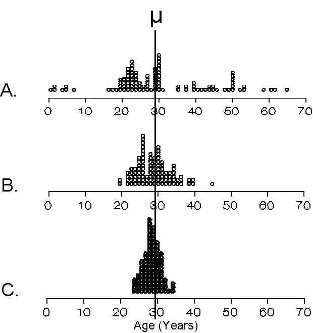
With this in mind, let us consider three sampling experiments based in the sampling frame listed as http://www.sjsu.edu/faculty/gerstman/StatPrimer/populati.htm. This population consists on 600 individuals (N = 600) with a mean (�) AGE of 29.5 and standard deviation (s) of 13.6. Notice use of � and s to indicate that these are the population mean and standard deviation, respectively.
The figure to the right shows three sampling experiments based in this
population.
Sampling distribution A shows 100 AGE values chosen at random. This can be viewed as a distribution of sample means in which each sample has n = 1.
Sampling distribution B shows 100 independent sample means, each based on n = 10. That is, the experimenter took 100 simple random samples from the population and calculated and calculated 100 means based on these independent random samples.
Sampling distribution C shows 100 sample means each based on n = 30. One-hundred new random samples each having 30 observations were used to calculate these 100 means.
Based on these results we note:
(1) With increasing sample size from n = 1 to n = 10 to n = 30, the sampling distribution becomes increasingly bell-shaped. This is the basis of The Central Limit Theorem.
(2) Each distribution is centered on population mean �. This is the basis of the unbiasedness of the sample mean.
(3) With increasing sample size, the sampling distribution tends to cluster more tightly around the population mean. This is the basis of the Law of Large Numbers.
These three postulates form the basis of sampling theory. Let us review each in turn.
The central limit theorem postulates that distributions of sample means tend toward normality even when the initial variable is skewed or non-normal. This finding strengthens as n increases. That is, the normality of the sampling distribution of a mean is more assured when working with large samples. An often repeated rule-of-thumb is that the normality can be assumed if n >= 30. This important finding justifies the use of statistical procedures based on normal distribution theory even when working with non-normal variables.
This postulate suggests that the average of a sampling distribution of means is the population mean. An unbiased estimator will have an expected value equal to the parameter it is trying to estimate. Since the expected value of the sample mean (x) is the population mean, it is an unbiased estimator of �. This is reflected in the fact that all three sampling distributions illustrated above are more-or-less centered on �.
This postulate states that distributions of sample means based on large samples cluster more tightly around � than sample means based on small samples. In other words, means from large samples are more precise than means from small samples. This also suggests that the precision of a sample mean can be quantified in terms of the spread (standard deviation) of the sampling distribution. The standard deviation of the sampling distribution then determines the standard error of the mean.
The standard error of a mean is a statistic that indicates how greatly a particular sample mean is likely to differ from the population mean. It is, in fact, the standard deviation of the hypothetical sampling distribution of the mean.
We have two formulas for the standard errors of a mean. One formula is used when the population standard deviation is known. Let us use the acronym SEM to indicate this standard error. The formula for this statistic is:
SEM = s / sqrt(n)
where s represents the population standard deviation, "sqrt" represents "the square root of", and n represents the sample size. For example, for a variable with s = 13.586 and a sample size of n = 10, SEM = 13.586 / sqrt(10) ~= 4.3.
When the population standard deviation is not known it must be estimated) on the standard deviation in the sample (s). In such instances, let us use small case letters to represent the standard error of the mean (sem). The formula is now:
sem = s / sqrt(n)
For example, when the sample standard deviation (s) = 16 and n = 10, sem = 16 / sqrt (10) ~= 5.06.
Notice that the operations specified in the first and second formulas are the same. However, the first is based on an assumed ("known") population standard deviation, whereas the second formula is based on a calculated (sample) standard deviation.
Regardless of which standard error formula is used, it is worth noting that the standard error of a mean depends on:
Variables having high standard deviation tend to have high standard errors. In addition, means based on small samples tend to have high standard errors.
Statistical inference is the act of generalizing from a sample to a population with calculated degree of certainty. Whenever we face the difficult task of making sense of numbers we are in fact using a method of inference based on induction (Fisher, 1935. p. 39).
There are two traditional forms of statistical inference. These are:
Estimation provides a "guesstimate" of the probable location of the parameter you are trying to infer. Hypothesis testing provides a way to assess the "statistical significance" of a finding. Examples of each will help illustrate their use.
It is common for epidemiologists to want to learn about the prevalence of a condition -- smoking for instance -- based on the prevalence of the condition in a sample. In a given sample, the final inference may be "25% of the population above age 18 smokes" (point estimation). Alternatively, the inference may take the form that "between 20% and 30% of the population smokes" (interval estimation). Finally, the epidemiologist might simply want to test whether smoking rates have changed over time. In such instances, a simple "yes" or "no" conclusion would suffice (hypothesis testing).
Regardless of the inferential method being used, it is important to keep clearly
in mind the distinction between the parameters being inferred and the statistics
used to infer them. Parameters are population-based characteristics that you
wish to know. Statistics are numerical summaries of the sample. Although the
two are related, they are not interchangeable. Parameters are unknown;
Statistics are calculated. Parameters are hypothetical; Statistics are observed.
Parameters are constants; Statistics are random variables. Therefore, we use
different symbols to represent parameters and statistics. For example, � is
used to represent the population mean (the parameter) and x is used to
represent the sample mean (the statistic). 
Estimation comes in two forms:
Point estimation provides the single best "guestimate" of the parameter's location. For example, sample mean x is the point estimator of population mean (�).
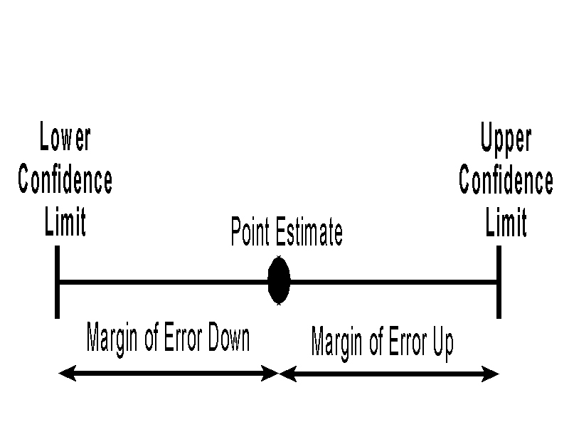 Interval estimation surrounds the point estimate with a margin of
error, thus forming a confidence interval. Confidence intervals are
usually constructed at the 95% level of confidence, although other
levels of confidence are possible (e.g., 90% confidence intervals, 99%
confidence intervals).
Interval estimation surrounds the point estimate with a margin of
error, thus forming a confidence interval. Confidence intervals are
usually constructed at the 95% level of confidence, although other
levels of confidence are possible (e.g., 90% confidence intervals, 99%
confidence intervals).
It is important to note that not all confidence intervals for � will capture the population mean. By design, only 95% of 95% confidence interval will capture the parameter. It follows that 5% of 95% confidence intervals for � will fail to capture the parameter. One never knows for certain.
Because sampling distributions of means tend to be normally distributed (central limit theorem) with an expected value of � (unbiasedness of the sample mean) and standard error (SEM) = s/n, approximately 95% of sample means will lie within �1.96 SEMs of �. In symbols:
Pr[� (1.96)(SEM) < x < � + (1.96)(SEM)] = .95.
Notice that this formula applies only when the exact SEM is used and s is known.
From algebra, it follows:
Pr[ x + (1.96)(SEM) > � > x (1.96)(SEM)] = .95
Therefore, a 95% confident interval for � is given by:
x � (1.96)(SEM)
For example, a 95% confidence interval for data in which x = 29.0, s = 13.586, and n = 10 (so SEM = 13.586 / sqrt(10) = 4.30), is equal to 29.0 � (1.96)(4.30) = 29.0 � 8.428 = (20.6, 37.4).
Notice that the confidence interval formula is of the form:
(point estimate) � (confidence coefficient)(standard error)
This will become important in other contexts.
The above formulation assumes that the population standard deviation is known. When the population standard deviation is not known, it must be estimate from the sample with s, and Student's adaptation of the normal distribution is used to provide the confidence coefficient for the confidence interval. A formula for a (1 - a)100% confidence interval for � when s is not know is:
x � (tdf,1-a/2)(sem)
where sem = s / n and tdf,1-a/2 represents the 1 - a/2 percentile on a t distribution with n - 1 degrees of freedom .
For example, suppose that we have the 10 AGE values as follows:
52, 50, 42, 24, 11, 27, 5, 21, 28, 30
The sample mean (x) = 29.00, the sample standard deviation (s) = 15.40, and n = 10. The estimate of the standard error of the mean (sem) = 15.40 / (10) = 4.87. The 95% confidence interval for � = 29.00 � (t9,.975)(4.87) = 29.0 � (2.26)(4.87) = 29.00 � 11.01 = (17.99, 40.01).
Web Calculators: Several web calculators perform confidence interval calculations for � (e.g., http://www.ed.asu.edu/mci.html)
SPSS Computation: SPSS calculates confidence intervals for means when the Statistics | Summarize | Explore command is issued.
In collecting data for a survey, one obvious question is "How big a sample is needed?" This depends, in part, on the required precision of the study.
Let d represent an acceptable margin of error in estimating �. This margin or error is equal to half the confidence interval's length and is about equal to twice the standard error of the mean:
d ~= (2)(sem)
A sample size that will achieve margin of error d with good reliability when calculating a 95% confidence interval for � is given by the formula:
n = 4s2/d2
For example, to estimate � with margin of error (d) = 5 for a variable with a standard deviation of s = 15, the required sample size is n = (4)(152)/52 = 36. In contrast, to estimate the same population mean with margin of error (d) = 2.5, we would need n = (4)(152)/(2.5)2 = 144. Notice that this second study would require four times the sample size of the first.
Sampling distribution of a mean: the hypothetical frequency distribution of sample means that would occur from repeated independent samples of size n from the population.
Central Limit Theorem: an axiom that states that distributions of sample means will tend toward normality, even if the initial variable is non-normal.
Unbiased estimate: an estimate from a sample which has an expected value that is equal to the parameter it is trying to estimate.
Law of large numbers: an axiom that states that the accuracy of a sample mean increases as the numbers studied increases, and that large samples are more likely to be representative of the "universe" than small samples.
Standard error of the mean (SEM): a statistic that indicates how greatly a particular sample mean is likely to differ from the mean of the population; SEM = s / /n
Estimated standard error of the mean (sem): the standard error of the mean statistic based on a sample variance or standard deviation; sem = s / /n
Margin of error (d): a "± value" that the statistician draws around the estimate in order to locate the probable location of the parameter being estimated, usually set to be about twice the size of standard error of the estimate, so that 95% of estimates will fall within this range; d = (2)(sem).