Background
Scatter Plot
Correlation
Regression
Importance of Visualization
Review Questions
References
Correlation and regression are complex and powerful statistical techniques that have wide application in data analysis. We will just address the tip of the iceberg for this topic, by basic linear correlation and regression techniques. This is used to analyze the relationship between two continuous variables. In general, the dependent (outcome) is referred to as Y and the independent (predictor) variable is called X.
To illustrate both methods, let us use the data set called BICYCLE.SAV. Data come from a study of bicycle helmet use (Y) and socioeconomic status (X). Y represents as the percentage of bicycle riders in the neighborhood wearing helmets. X represents the percentage of children receiving free or reduced-fee meals at school. Data are:
|
School Neigborhood |
X (% receiving meals) |
Y (% wearing helmets) |
|
Fair Oaks |
50 |
22.1 |
|
Strandwood |
11 |
35.9 |
|
Walnut Acres |
2 |
57.9 |
|
Discov. Bay |
19 |
22.2 |
|
Belshaw |
26 |
42.4 |
|
Kennedy |
73 |
5.8 |
|
Cassell |
81 |
3.6 |
|
Miner |
51 |
21.4 |
|
Sedgewick |
11 |
55.2 |
|
Sakamoto |
2 |
33.3 |
|
Toyon |
19 |
32.4 |
|
Lietz |
25 |
38.4 |
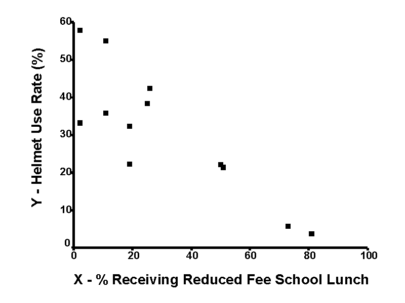
The basis of both correlation and regression lies in bivariate ("two variable") scatter plots. This type of graph shows (
xi, yi) values for each observation on a grid. The scatter plot of the illustrative data set is shown below:
Notice that this graph reveals that high
X values are associated with low values of Y. That is, as the number of children receiving reduced-fee meals at school increases, the bicycle helmet use rate decreases. Thereby, a negative correlation is said to exist.In general, scatter plots may reveal a:
SPSS: To draw a scatter plot with SPSS, click on
Observations that do not fit the general data pattern are called
outliers. Identifying and dealing with outliers is an important statistical undertaking. In some instances, outliers should be excluded before analyzing the data and in other instances they should remain present during analysis. However, they should never be entirely ignored. For insights into how to address outliers, please see www.tufts.edu/~gdallal/out.htm.
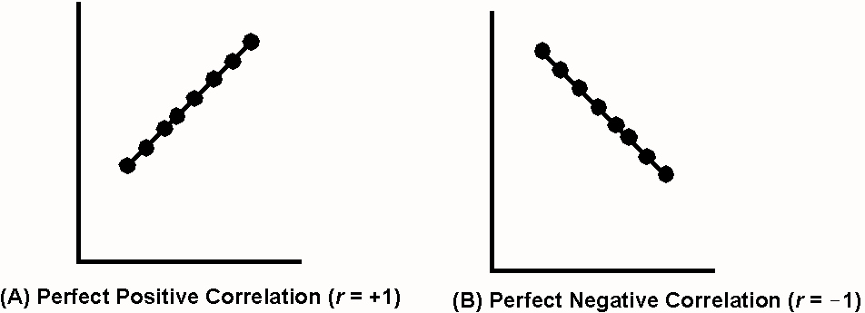
Pearson's correlation coefficient
(r) is a statistic that quantifies the relationship between X and Y in unit-free terms. The closer the correlation coefficient is to +1 or -1, the better the two variables "keep in step." This can be visualized by the degree to which the scatter cloud adheres to an imaginary trend line through the data. When all points fall on a trend line with an upward slope, r = +1. When all points fall on a downward slope, r = -1.
Perfect positive and negative correlations, however, are seldom encountered, with most correlations coefficients falling short of these extremes. We may judge the strength of the correlation in qualitative terms: the closer
r is to-1 or +1, the stronger is the correlation..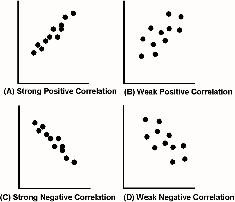
Although there are no firm cutoffs for strength, let us say that absolute correlations |
r| greater than or equal to 0.7 are "strong." Absolute correlations less than 0.3 are "weak." Absolute correlations between 0.3 and 0.7 are moderate.|
Absolute value of r |
Strength of correlation |
|
< 0.3 |
weak |
|
0.3 - 0.7 |
moderate |
|
> 0.7 |
strong |
To calculate correlation coefficients, we need to calculate various sums of products and cross-products. There are three types of sums of squares.
The sum of squares around the mean of the X variable (
ssxx) as:ssxx
= S(xi - x)�This statistic measures the spread of independent variable
X, and is the numerator of formula for the variance of X.For the illustrative data set, x = 30.833 and
ssxx = 7855.67.The sum of squares around the mean of the Y variable (
ssyy) as:ssyy
= S(yi - "y bar")�This statistics measures the spread of dependent variable Y. It is the numerator of the formula for the variance of Y.
For the illustrative data set, "y bar" = 30.883 and
ssyy = 3159.68.Finally, let us define the sum of the crossproducts (
ssxy) as:ssxy
= S(xi - x)(yi - "y bar")This statistic is analogous to the above sum of squares, but instead quantifies the
covariance between the independent variable X and dependent variable Y.For the illustrative data set,
ssxy = -4231.1333.The formula for the correlation coefficient is:
r
= (ssxy) / sqrt(ssxx * ssyy)For the illustrative data set,
ssxy = -4231.1333, ssxx = 7855.67, ssyy = 3159.68. Therefore, r = (-4231.1333) / sqrt(7855.67 * 3159.68) = -0.849. This suggests a strong negative correlation between X and Y.Comment: Although there is no firm cutoff for what constitutes a strong correlation, let us say that |r| > 0.70 can be assumed to suggest a strong correlation.
SPSS: To compute correlation coefficients with SPSS, click onStatistics | Correlate | Bivariate, and then select the variables you want to analyze.
The primary goal of regression is to draw a line that predicts the average change in
Y per unit X. If all data points were to fall exactly on a straight line, this would be a trivial matter. However, because most points will not fall exactly on the line, choosing a line for statistical inferences is a complicated endeavor.To decide on the "best" line that describes the data, we model the expected value of
Y for a stated value of X (E(Y|x)) so that:E
(Y|x) = a + bxwhere a represents the intercept of the line and b represents the line's slope.
In recognizing the above equation as an equation for a line, the intercept (a) is where the line crosses the
Y axis and the slope (b) represents the incline of the line (change in Y per unit X). To determine the intercept and slope of the regression line, we measure the distance of each data point from the line. This is called the residual, represented with the symbol ei ("epsilon"). Each data point can now be represented with the equation:Yi
= a + bx + eiOur strategy is to determine the regression line that minimizes the sum of the squared residuals (min Se�). This is the
least squares criterion.The parameter b is called the regression coefficient, or the slope of the regression line. The best estimate of this slope, denoted
b, is given by the formula:b =
ssxy / ssxxwhere
ssxy represents the sum of the crossproducts (see above) and ssxx represents the sum of the squares for variable X.For the illustrative data set,
ssxy = -4231.1333 and ssxx = 7855.67. Therefore b = -4231.1333 / 7855.67 = -0.54. This negative slope indicates that each unit of X is associated with a 0.54 decrease in Y, on average.SPSS: The regression coefficient and other regression statistics is computed by clickingStatistics | Regression | Linear. The regression coefficient slope is listed as the "Unstandardized Coefficients" for the X variable.
A given slope may describe any of an infinite number of parallel lines. To uniquely identify the line in question, an intercept is calculated.
Let a represent the intercept parameter, and let
a represent the estimate of this parameter. The estimate of the intercept is calculated by the equation:a
= "y bar" - bxwhere "y bar" represents the average of all Y values, b represents the slope estimate, and x represents the average of all X values.
For the illustrative data set, "y bar" = 30.8833, b = -0.54, and x = 30.8333. Therefore, a = (30.8833) - (-0.54)(30.8333) = 47.49.
SPSS: The intercept is computed by the Statistics | Regression | Linear command and is listed as the "Unstandardized Coefficients" for the "(Constant)."
Knowing the intercept and slope allows us to predict the value of Y at a stated value of X. Let y^ ("y hat") represent this predicted value. From the regression equation we know:
y
^ = a + bxThe regression model for the illustrative data set is: Predicted percent of bicycle riders wearing helmets(
y^i) = 47.49 + (-0.54)xi. So, for a neighborhood in which half the children receive free- lunches (X = 50), the expected helmet use rate y^ = 47.49 + (-0.54)(50) = 20.5.The standard error of the regression represents the standard deviation of
Y after taking into account its dependency on X. It quantifies the accuracy with which the fitted regression line predicts the relationship between Y and X. Let us use the symbol sY�X to denote this statistic.This statistic can be calculated in a number of different ways. Given our current state of knowledge, let us use the formula:
sY�X
= sqrt[(ssyy - b * ssxy) / (n - 2)]where
ssyy represents the sum of squares of Y, b represents the slope estimate, ssxy represents the cross-product, and n represent the sample size. For the illustrative data set, sY�X = 9.38.Let se represent the standard error of the slope estimate. It can be shown that:
seb
= sY�X / sqrt(ssxx)where
sY�X represents the standard error of the regression and x represents the deviation of an X value from the mean of all X's (i.e., x = xi - x).For the illustrative data set,
sY�X = 9.38 and ssxx = 7855.67. Thereby, seb = 9.38 / sqrt(7855.67) = 0.1058.For a 95% confidence interval for b, we calculate:
b
� (tn-2,.975)(seb)For the illustrative data set, we have -0.54 � (
t10,.975)(0.1058) = -0.54 � (2.23)(0.1058) = -0.54 � 0.24 = (-0.30, - 0.78). Notice how this confidence interval excludes a possible slope of 0 with 95% confidence.Because the straight-line dependency in the sample may not necessarily hold up in the population, we have adopt different notation to represent the sample regression coefficient (b) and its regression coefficient parameter (b). We test the sample slope for significance by performing the test:
H
0: b = 0This can be tested with the statistic
t-stat = b / (seb)
where b represents the estimate for the regression coefficient parameter and se represents the standard error of the regression coefficient. This statistic has n - 2 degrees of freedom. The current example shows t-statistic = -0.54 / .1058 = -5.10 with 12 - 2 = 10 degrees of freedom. This translates to p (two-sided) < .0005. Using APA notation, this is denoted t(10) = -5.09, p < .0005.
Comment: We will not cover the ANOVA table produced by SPSS.
Inference about regression estimates requires the following assumptions:
Notice how these assumptions form the mnemonic "LINE."
The linearity assumption can be assessed when viewing the scatter plot.
The independence assumption suggests data are selected randomly, so that everyone in the population has an equal probability of entering the sample, and so that selection of one individual does not influence the probability of selecting any other.
The normality and equal variance assumptions can be understood by scrutinizing the residual error terms. Let us represent the residual error term associated with point (xi, yi) with the symbol ei. Now each data point can be described by the equation y^i = a + bxi + ei,, where y^i represents the predicted value of Y given an intercept of a and slope of b. Under the null hypothesis, residual error terms are normally distributed with a mean of zero and constant variance. In symbols, e ~ N(0, sigma-squared). Figure 9 illustrates this assumption graphically.
Comment: SPSS has powerful software tools to help address regression assumptions, but these will not cover in this class. (A separate regression course would be necessary.)
In addition to the "LINE" assumptions needed for valid regression inference, correlational inferences assumes that the joint distribution of
X and Y are normality (bivariate normal population). Figure 10 shows a bivariate normal population.Comments:
In the space of one hundred and seventy-six years the Lower Mississippi River has shortened itself two hundred and forth-two miles. This is an average of a trifle over one mile and third per year. Therefore, any calm person, who is not blind or idiotic can see that in the Old Oölitic Silurian period, just a million years ago next November, the Lower Mississippi River was upward of one million three hundred thousand miles long, and stuck out over the Gulf of Mexico like a fishing rod. And by the same token any person can see that seven hundred and forty-two years form now, the lower Mississippi will be only a mile and three-quarters long, and Cairo [Illinois] and New Orleans will have joined their streets together, and be plodding comfortably along under a single mayor and a mutual board of aldermen.
Without visualizations of the scatter plot, nonsensical regression results can and often do result. Careful review of the scatter plot can avoid such nonsense. Take, for instance, the data sets known as Anscombe's quartet (1973), shown below:
TABLE: Anscombe's Quartet
|
Data Set I |
Data Set II |
Data Set III |
Data Set IV |
||||
|
X |
Y |
X |
Y |
X |
Y |
X |
Y |
|
10.0 |
8.04 |
10.0 |
9.14 |
10.0 |
7.46 |
8.0 |
6.58 |
Each of these data set has identical correlation and regression statistics (
a = 3, b = 0.5, r = +0.82, p = .00217, etc.). However, scatter plots reveal clearly different relationships in each instance, with data set 1 showing a clear regression trend, data set 2 showing an upside-down U-shape, data set 3 showing a perfectly fitting algebraic line with one outlier, and data set 4 shows a bizarre vertical pattern with one outlier. (Try plotting each of these data sets!) Clearly, then, the regression equation y^ = 3 + 0.5x should not be used to represent these four very different relationships.Y
= dependent variable1. A straight line is defined by its slope and intercept. What does the slope represent? What does the intercept represent?
ANS: The slope represents the angle of the line (i.e., the change in Y per unit X). The intercept represents the point at which the line crosses the Y-axis.
2. What differentiates a statistical linear equation from an algebraic one?
ANS: Statistical equations have an error term to capture the random scatter around the line. Algebraic equations have no error term, since each data point falls exactly on the line.
3. What does a slope of zero indicate?
ANS: A zero slope indicates no correlation between X and Y.
4. What does the correlation coefficient represent?
ANS: The correlation coefficient measures the "fit" of data points around a trend line. The closer the correlation coefficient is to +1 or -1, the more closely data adhere to the line.
5. When we refer to the normality assumption of regression, to what are we referring?
ANS: We are referring to the distribution of the "residuals" (ei).
6. What symbol is used to denote statistical estimator of the slope? What symbol is used to denote the slope parameter?
ANS: Estimator: b. Parameter: b
7. What symbol is used to denote the correlation coefficient estimator? What symbol is used to denote the correlation coefficient parameter?
ANS: Estimator: r. Parameter: [Greek letter] "rho"
8. A
t statistic can be used to test a slope. This statistic is associated with ___ degrees of freedom.ANS: n - 2
9. Negative slopes suggest that as
X increases, Y tends to _______________.ANS: decrease
Absombe, F. J. (1973). Graphs in statistical analysis. American Statistician, 27, 17-21.
Berk K. N. (1994). Data Analysis with Student SYSTAT. Cambridge, MA: Course Technology.
Dean, H. T. (1942). Arnold, F. A., & Elvov, E.. Domestic water and dental caries. Public Health Reports, 57, 1155-1179.
Hampton, R. E. (1994). Introductory Biological Statistics. Deburque, IW: Wm. C. Brown.
Kruskal, W. H.(1960) Some remarks on wild observations. Technometrics Available:
www.tufts.edu/~gdallal/out.htm.Monder, H. (1986). [Alcohol consumption survey.]. Unpublished raw data.
Muddapur, M. V. (1988). A simple test for correlation coefficient in a bivariate normal population. Sanky: Indian Journal of Statistics. Ser. B. 50, 60-68.
Neter, J., Wasserman, W., & Kutner, M. H. (1985). Applied Linear Statistical Models (2nd Ed.) Homewood, IL: Richard D. Irwin.
Perales, D. & Gerstman, B. B. A bi-county comparative study of bicycle helmet knowledge and use by California elementary school children. The Ninth Annual California Conference on Childhood Injury Control, San Diego, CA, March 27-29, 1995.
Zar, J. H. (1996). Biostatistical Analysis. (3rd Ed.) Upper Saddle River, NJ: Prentice Hall.